Bayes’ rule is amazing. Ever since I came across Bayes’ rule in statistics I have been in love with this simple yet elegant formula in statistics which has application in wide area of research such as AI, health care, economics and what else. Although it looks very simple, in many cases it becomes very complicated to compute it in closed form. This complication arises due to the denominator of the formula which is the marginal probability distribution of the observations. This term is sometimes very hard (or virtually impossible) to compute analytically. To bypass this complexity, several approaches has been proposed to approximate the Bayesian posterior such as Variational inference, Markov Chain Monte Carlo (MCMC) etc . In this informal tutorial we are going to see how we can approximate the Bayes rule using MCMC.
Recap with an example
Before diving into the algorithm, just for revision let’s first see the Bayes’ rule with a linear regression example. Let’s say you are given 10 random values of \(x\) and their corresponding values of \(y\) from the quadratic function \(y = 2x^2 - 3x + 1\). Our goal is to guess the coefficients quadratic model \(w_0x^2 + w_1x + w_2\) using the given data (observations). This is an easy problem from machine learning perspective. We can simply do a least square regression with gradient descent to find an estimate of the coefficients \(w_0\), \(w_1\) and \(w_2\). However, this type of regression will give you only an fixed value estimate of these coefficients and thus you will have only a fixed function. Say for example, after the gradient descent we get \(w_0 = 1.87\), \(w_1 = -2.6\) and \(w_2 = 0.89\). Clearly, these values are not same as that of the actual function and these coefficient will not represent the actual function for all the possible values of x that were not in the given data set. The quadratic model with these estimated coefficients will predict \(y\) for any value of \(x\) with absolute certainty and this might not be very good for many practical purposes. Many times it is better to have an estimate of prediction uncertainty and with the prediction.
How to get an estimate of the prediction uncertainty? One way to deal with this is to have a probability distribution over the coefficients (say a multivariate Gaussian distribution with some mean and covariance) instead of fixed values. Then we can sample some set of \((w_0, w_1, w_2)\) from this distribution and then we can compute the \(y\) values using each set of \((w_0, w_1, w_2)\) for any value of \(x\). Thus we can have an estimate of mean and variance of predicted \(y\)s. The variance will correspond to the uncertainty in the prediction.
One way to estimate the probability distribution \(P(w_0, w_1, w_2)\) or simply \(P(W)\) is Bayesian inference i.e using Bayes’ rule. The Bayes’ rule can be written as follows:
\[P(W \mid D) = \frac{P(D \mid W)P(W)}{\int {P(D \mid W_i)P(W_i)dW_i}}\]where, \(W\) is the vector of coefficients of out quadratic model and \(D\) represents the given data.
\(P(W)\) : This is the prior distribution over \(W\). This is simply a guess (by us) or can be from some prior information about the model/problem.
\(P(W \mid D)\) : Probability distribution of \(W\) given the data \(D\) (i.e. the x,y pairs we were given) called posterior distribution over \(W\).
\(P(D \mid W)\) : This is called likelihood of the given data with some \(W\). This can be calculated form our model i.e the quadratic model. We’ll see it later how to do that.
\(\int {P(D \mid W_i)P(W_i)dW_i}\) : This is called the marginal distribution over the data. i.e the distribution of (x,y) pairs for all the possible values of \(W\) using our quadratic model. And this is the most problematic term in Bayes’ rule. For a complex model (such as neural networks) with continuos \(W\) it is very hard to compute this integral in closed form. And thus in those cases we cannot apply Bayes’s rule as it is and we need to approximate the posterior distribution from whatever portion of the formula is computable. One such approximation method is MCMC.
Now let’s jump into MCMC
In short the idea of MCMC is have a lot of \(W\)s from the posterior distribution \(P(W \mid D)\) and then estimating the distribution from the collected data. Wait wait wait…What!!!! How can we get samples from the posterior distribution \(P(W \mid D)\) without even computing it before? Is it not like the chicken and egg problem ? Well that’s the beauty of statistics I fall in love with everyday. We can actually have samples from \(P(W \mid D)\) without even computing it. Let’s see how:
Intuition behind MCMC
We can start with a random value of \(W\). Let’s call it \(W_{start}\). Then find another \(W\) (call it \(W_{next}\)) in the neighborhood of \(W_{start}\). Now compute the likelihood of the given data for them. If \(W_{next}\) has higher likelihood then use it as new \(W_{start}\). Otherwise reject \(W_{next}\) and get a new \(W_{next}\) in the neighborhood of \(W_{start}\). Repeat the process for quite a long time and we will reach the value of \(W_{start}\) that maximize the likelihood. This is like hill climbing. The problem is that this is just one value of \(W\) that maximizes the likelihood (i.e a good fit for the given). However, this approach can be used to have a large number of \(W\)s that comes from the posterior distribution.
Actual MCMC algorithm
STEP 1: As in the previous case, we start with a random value of \(W_{start}\). We define a multivariate Normal distribution \(\mathcal{N}\) with mean \(W_{start}\) and a fixed (user defined) co-variance \(\Sigma\) (called Proposal width).
STEP 2: Then we sample \(W_{next}\) from \(\mathcal{N}(W_{start}, \Sigma)\)
STEP 3: Compute
\[acceptance = \frac{P(W_{next} \mid D)}{P(W_{start} \mid D)} = \frac{P(D \mid W_{next})P(W_{next})}{P(D \mid W_{start})P(W_{start})}\]Thus we get the ratio of the posterior at \(W_{start}\) and \(W_{next}\) which is nothing but the ratio of the numerators of the Bayes’ rule.
STEP 4 acceptance is our probability of accepting \(W_{next}\) as new \(W_{start}\). So we draw a random number between 0 and 1 and if it is less than acceptance then we will replace \(W_{start}\) by \(W_{next}\).
STEP 5 Repeat the process from STEP 1 until convergence.
After sufficient number of iterations we start getting samples (\(W\)s) approximately from the actual posterior distribution. From these samples we can approximate the posterior distribution over \(W\) (let’s say with a Normal distribution).
And this is the end of the main story.
Practical considerations
Now if we look back, in the algorithm we have used mainly 2 ‘not so well’ defined terms:
- User defined covariance \(\Sigma\)
- “Convergence” of the process
Covariance \(\Sigma\) (Proposal width): This parameter should be tuned in such a way that acceptance rate at any time is approximately 50%. i.e 50% of the \(W_{next}\) should be accepted by the algorithm. This is important because if you use a very larger covariance (proposal width), then chance of accepting a jump wll be very small and the algorithm will be inefficient. On the other if proposal width is very small then it will take more time to converge.
Convergence: There is no perfect way to guess this. One simplest way is to observe the steadiness of the statistics of the drawn samples (e.g Converging mean/variance statistics to a value). A better way is to see the process graphically with trace (simply plotting the value over time) and density (smoothed histogram) plots for each variable (i.e dimensions of W). At convergence these plots should be approximately stable. Further readings here
Let’s run our example in Python
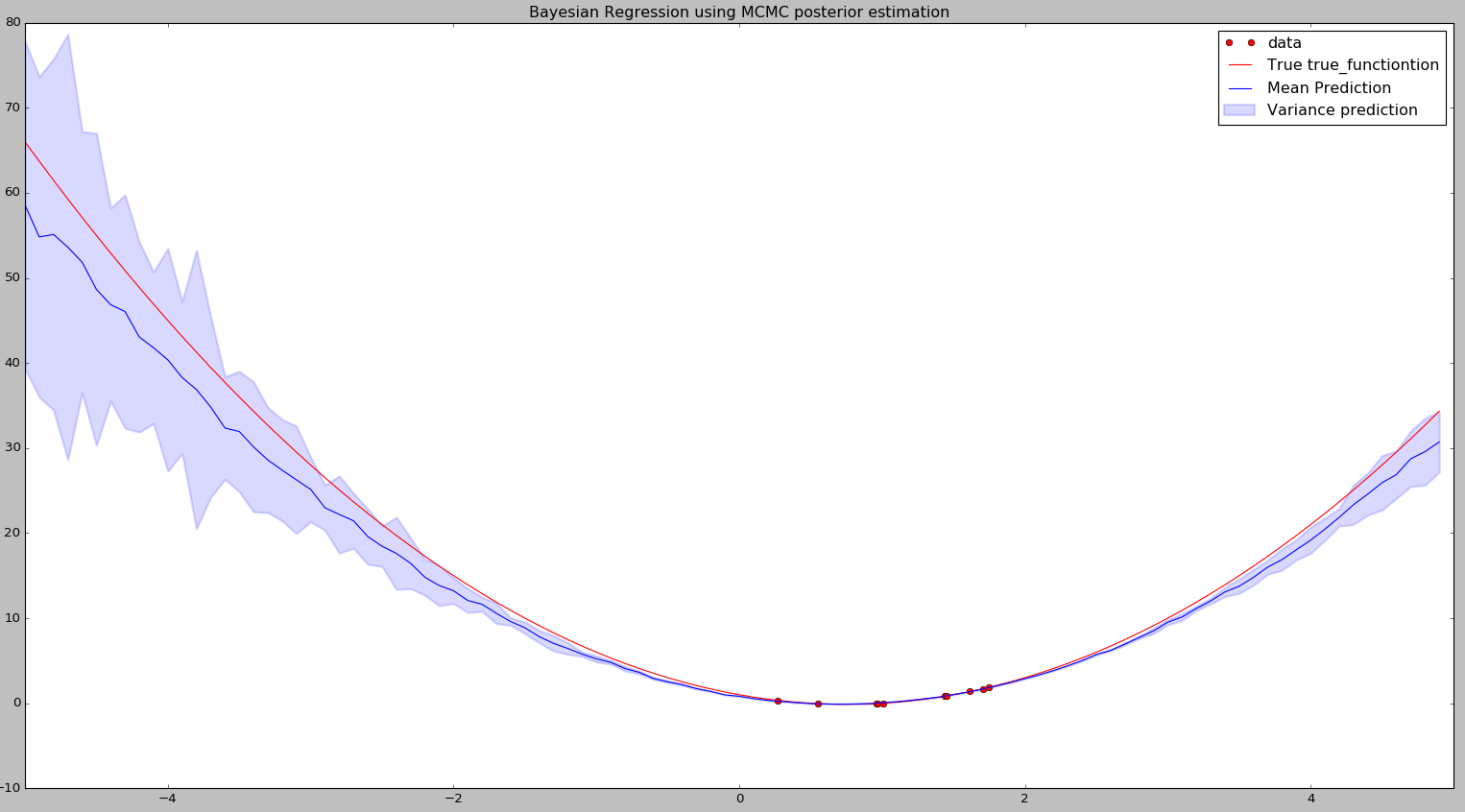
I have written a small and very straight forward code to find the values of \(W_0\), \(W_1\) and \(W_2\) for our linear (actually quadratic) regression example using Bayesian approach with approximation of the posterior using MCMC. After running this we should get \((W_0, W_1, W_2)\) very close to our actual coefficients (2, -3, 1). The code and the plot is shown below:
import numpy as np
from scipy.stats import multivariate_normal
import math
import matplotlib.pyplot as plt

def true_function(x):
    return 2*x**2 - 3*x + 1

prior_mean = np.array([0.,0.,0.])
prior_cov = np.array([[1.,0.,0.],[0.,1.,0.],[0.,0.,1.]])
variate = multivariate_normal(mean=prior_mean, cov=prior_cov)
def prior(w):
    return variate.pdf(w)

def model(x,w):
    return w[0]*x**2 + w[1]*x + w[2]

def likelihood(data_x, data_y, w):
    lik = 1.0
    output_var = np.array([0.01])
    for i in range(len(data_y)):
        output_mean = np.array([data_y[i]])
        var = multivariate_normal(mean=output_mean, cov=output_var)
        model_pred = model(data_x[i], w)
        lik = lik * var.pdf(model_pred)

    return lik

def mcmc_estimate(current_mean, sampling_covar, data_x, data_y):
    samples = []
    samples.append(current_mean)
    mean_w = []
    covar_w = []

    accepted_count = 0
    for i in range(10000):
        next_mean = np.random.multivariate_normal(current_mean, sampling_covar)
        numerator_bayes_current = likelihood(data_x,data_y, current_mean) * prior(current_mean)
        numerator_bayes_next = likelihood(data_x,data_y, next_mean) * prior(next_mean)
        acceptance = numerator_bayes_next/(numerator_bayes_current)

        r = np.random.rand(1)

        if acceptance > r:
            accepted_count += 1.0
            current_mean = next_mean
            samples.append(current_mean)

            if len(samples) > 1000:
                samples = samples[-1000:]
                mean_w = np.mean(samples,axis=0)
                covar_w = np.cov(samples,rowvar=False)

        if i%1000.0 == 0:
            print i,') mean_w: ', mean_w
            print 'Acceptance rate: ', accepted_count/(i+1)
            # print i,')cov_w: ', covar_w


    return mean_w, covar_w

#Generate some random inputs
data_x = np.random.rand(10)*2.0
#Compute the outputs using the true true_functiontion
data_y = [true_function(k) for k in data_x]


#Set the initial mean to sample w from
current_mean = np.array([0.0, 0.0, 0.0])
#Set the fixed covariance for w to be sampled from
#The covariance should be tuned in such a way that acceptance rate is around 0.5
sampling_covar = np.array([[0.001,0.,0.], [0.,0.001,0.], [0.,0.,0.001]])
#Estimate mean and covar w using mcmc
mean_w, covar_w = mcmc_estimate(current_mean, sampling_covar, data_x, data_y)

#Plot the given data points
plt.plot(data_x,data_y, 'or', label='data')

#Plot the true true_functiontion
x = np.arange(-5,5,0.1)
y = [true_function(k) for k in x]
plt.plot(x,y, '-r', label='True true_functiontion')

#Plot the learned true_functiontion
#For every input, query the model using sampled w from learned mean and covar
#Then compute mean prediction and prediction variance
ymean = []
yh = []
yl = []
for i in range(len(x)):
    input = x[i]
    output = []
    for j in range(30):
        w = np.random.multivariate_normal( mean_w, covar_w)
        output.append(model(input,w))

    m = np.mean(output,axis=0)
    v = np.var(output, axis=0)
    ymean.append(m)
    yh.append(m+v)
    yl.append(m-v)

plt.plot(x,ymean, '-b',label='Mean Prediction')
plt.fill_between(x,yh, yl, alpha=0.15, linewidth=2, color='blue', label='Variance prediction')
plt.legend()
plt.title("Bayesian Regression using MCMC posterior estimation")
plt.xlim([-5,5])
plt.show()